Microsoft Excel: Concatenation (Concat)
Microsoft Excel: Concatenation (Concat)
Concatenation – What is it?
The CONCAT function is one of Excel’s text functions. It is used to join two or more columns of text from multiple ranges and/or strings, but it doesn’t provide delimiter or IgnoreEmpty arguments.
So what does that mean?
Well, if we have multiple columns with text, and we want to combine the text into one column, we would use the CONCAT function.
CONCAT replaces the CONCATENATE function. However, the CONCATENATE function will stay available for compatibility with earlier versions of Excel.
How to Concatenate
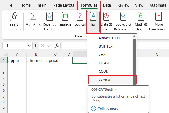
Using the CONCAT function, select an empty space where data is to be displayed; i.e. not part of one of the existing columns of data.
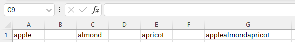
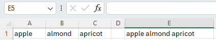
For the example we will use this data set: Column: A: apple | B: almond | C: apricot
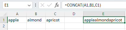
Using the CONCAT function; Column E would appear as: applealmondapricot – containing the data from all three cells into one cell.
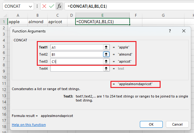
We will use the function wizard to define the function arguments, entries consist of A1,B1,C1.
Clicking OK will provide the list of the concatenated sum.
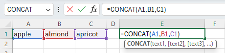
However, if we click into the cell (double click or press F2); it will only show the formula; it is not an actual value.
*Notice above that the arguments do not include any spaces, merging all of the words together. There would need to be spaces after each word in each column for the results to look like below:
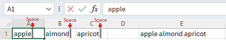
Even if you include empty columns between the data range, it does not count as spaces.
CONCAT vs. CONCATENATE
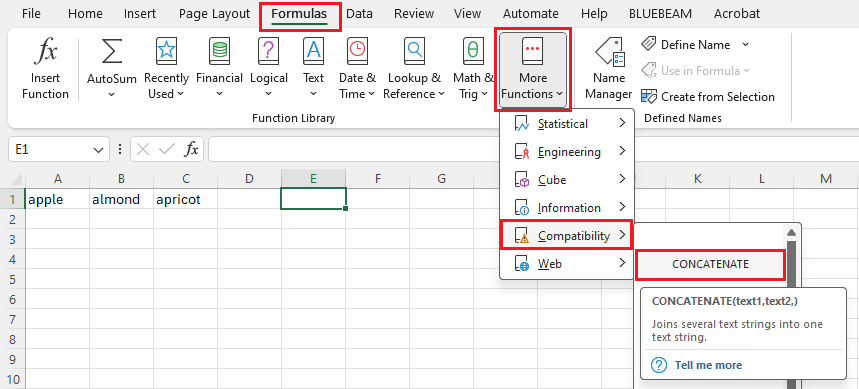
For older versions of Excel or older spreadsheet versions (.xls), you can use the More Functions, Compatibility, CONCATENATE function. Which functions similarly to the CONCAT formula.
Important: In Excel 2016, Excel Mobile, and Excel for the web, this function has been replaced with the CONCAT function. Although the CONCATENATE function is still available for backward compatibility, you should consider using CONCAT from now on. This is because CONCATENATE may not be available in future versions of Excel.
Important: In Excel 2016, Excel Mobile, and Excel for the web, this function has been replaced with the CONCAT function. Although the CONCATENATE function is still available for backward compatibility, you should consider using CONCAT from now on. This is because CONCATENATE may not be available in future versions of Excel.
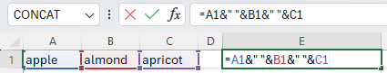
Another way to concatenate without using the wizard is with an Ampersand
The fastest and easiest method for joining the data in two or more cells is to use the ampersand. Yes, this little symbol works just as efficiently as the CONCAT functions. Just enter the formula like this: =A1&” “&B1&” “&C1. This simple formula joins the contents of Cell A1 with the contents of cell B1, with a space between the two so the results are apple almond apricot. The quotation space quotation is what keeps from merging the words.
Below are additional examples of what you can do with the CONCAT formula:
Data | First Name | Last Name |
brook trout | Andreas | Hauser |
species | Fourth | Pine |
32 | ||
Formula | Description | Result |
=CONCAT(“Stream population for “, A2,” “, A3, ” is “, A4, “/mile.”) | Creates a sentence by joining the data in column A with other text. | Stream population for brook trout species is 32/mile. |
=CONCAT(B2,” “, C2) | Joins three things: the string in cell B2, a space character, and the value in cell C2. | Andreas Hauser |
=CONCAT(C2, “, “, B2) | Joins three things: the string in cell C2, a string with a comma and a space character, and the value in cell B2. | Hauser, Andreas |
=CONCAT(B3,” & “, C3) | Joins three things: the string in cell B3, a string consisting of a space with ampersand and another space, and the value in cell C3. | Fourth & Pine |
=B3 & ” & ” & C3 | Joins the same items as the previous example, but by using the ampersand (&) calculation operator instead of the CONCAT function. | Fourth & Pine |
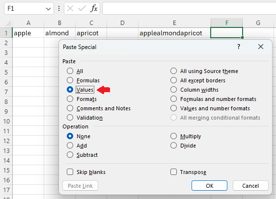
Converting formula output to Values
If we can Copy and Paste Special into a different cell; selecting Values as the paste option, it will provide the merged data rather than the formula.
Related Articles
Microsoft Excel: How to Add a Watermark to a Worksheet
Microsoft Excel: How to Add a Watermark to a Worksheet Do you still think that you can’t add a watermark to your Excel worksheet? I have to say that you are all abroad. You can mimic watermarks in Excel 2019, 2016, and 2013 using the HEADER & FOOTER ...Microsoft Excel: How to select alternate columns
Microsoft Excel: How to select alternate columns This article will guide you step-by-step through the process of selecting specific columns in Excel, such as every other or every nth column. Microsoft Excel, the go-to spreadsheet software for data ...Microsoft Excel: Text to Columns
Microsoft Excel: Text to Columns Data imported from other spreadsheets or databases is already separated into fields, using something called a field delimiter: a comma, tab, space, or custom character – to separate one field from another. These ...Microsoft Excel: How to make Drop-down lists
Microsoft Excel: How to make Drop-down lists In Excel 365, they’ve added the ability to search within data validation lists, which is a huge time-saver when working with large sets of data. However, even with this new option, out-of-the-box Excel ...Microsoft Excel: Turn table headers on or off
Microsoft Excel: Turn table headers on or off When you create an Excel table, a table Header Row is automatically added as the first row of the table, but you have to option to turn it off or on. When you first create a table, you have the option of ...