Microsoft Excel: How to Add a Watermark to a Worksheet
Microsoft Excel: How to Add a Watermark to a Worksheet
Do you still think that you can’t add a watermark to your Excel worksheet? I have to say that you are all abroad. You can mimic watermarks in Excel 2019, 2016, and 2013 using the HEADER & FOOTER TOOLS.
It often happens that you need to add a watermark to your Excel document. The reasons can be different. One of them is just for fun, as I’ve done for my work timetable.

I’ve added an image as a watermark to my timetable. But most commonly you can come across the documents labelled with such text watermarks as “Confidential“, “Draft“, “Restricted“, “Sample“, “Secret“, etc. They help to underscore the status of your document.

Unfortunately, Microsoft Excel 2016-2010 doesn’t have a built-in feature to insert watermarks in worksheets. However, there is a tricky method that allows you to mimic watermarks in Excel using the HEADER & FOOTER TOOLS and I’m going to share it with you in this article.
Create a watermark image
The first thing you need to do is to create a watermark image that will later appear on the background of your worksheet. You can do it in any drawing program (for example, in Microsoft Paint). But for simplicity, I’ve created an image right in a blank Excel worksheet using the WordArt option.

If you are curious how I’ve done it, see detailed instructions below.
- Open a blank worksheet in Excel.
- Switch to Page Layout view (go to VIEW – > Page Layout in the Ribbon or click the “Page Layout view” button on the Status bar at the bottom of your Excel window).
- Click the WordArt icon in the Text group on the INSERT tab.

- Select the style.
- Type the text that you want to use for the watermark.
Your watermark image is almost ready, you just need to resize and rotate it to make it look good. What are the next steps?
- Make the background of your WordArt object clear, i.e. untick the Gridlines check box in the Show group on the VIEW tab
- Click on the image twice to select it
- Right-click once and choose “Copy” from the menu
- Open MS Paint (or the drawing program you prefer)
- Paste the copied object into the drawing program
- Press the Crop button to get rid of extra space from your image
- Save your watermark image as either a PNG or GIF file
Now you are set for inserting the created and saved image into the header as described below.
Add a watermark to the header
Once you’ve created your watermark image, the next step is to add the watermark to your worksheet header. Whatever you put in your worksheet header will automatically print out on every page.
- Click on the INSERT tab in the Ribbon
- Go to the Text section and click on the Header & Footer icon

Your worksheet automatically switches to the Page Layout view and a new HEADER & FOOTER TOOLS tab appears in the Ribbon.
- Click on the Picture icon to open the Insert Pictures dialog box

- Browse for an image file on your computer or use Office.com Clip Art or Bing Image, which you want to have as a watermark in your Excel sheet.
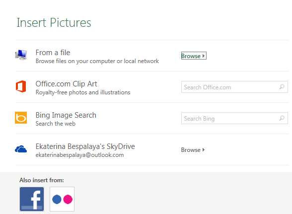
- When you’ve found the desired image, select it and press the Insert button. The text &[Picture] now appears in the header box. This text indicates that the header contains a picture.
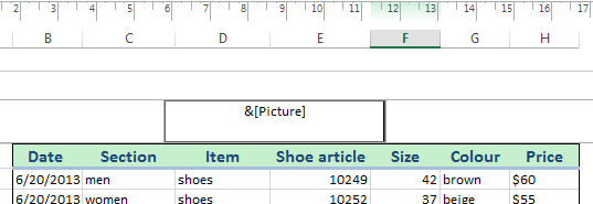
You still don’t see a watermark in your worksheet.
Click within any cell out of the header box to see what the watermark looks like.

Now when you click on another page in your worksheet, the watermark will be automatically added to that page as well.
REMEMBER that watermarks are visible only in Page Layout view, in the Print Preview window and on the printed worksheet. You cannot see watermarks in the Normal view, which most people use when they work in Excel 2010, 2013 and 2016.
Format your watermark
After you add your watermark image you’ll likely be keen to resize or reposition it. You can also remove it if you’ve had enough of it.
Reposition a watermark
It is a common thing that the added image turns out to be at the top of the worksheet. Don’t worry! You can easily move it down:
- Go to the header section box
- Place your cursor in front of &[Picture]
- Press the Enter button once or several times to get the watermark centered on the page
You may experiment a bit to achieve the desirable position for the watermark.
Resize a watermark
- Go to INSERT – > Header & Footer again.
- Choose the Format Picture option in the Header & Footer Elements group.
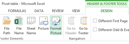
- To change the size or scale of your picture, click the Size tab in the open window.
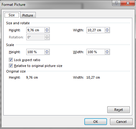
- Choose the Picture tab in the dialog box to make color, brightness or contrast changes.
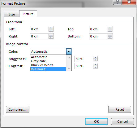
I recommend using the Washout feature from the dropdown menu under Image Control as it makes the watermark fade out and it becomes easier for users to read the content of the worksheet.
Remove a watermark
- Click on the header section box
- Highlight the text or the picture marker &[Picture]
- Press the Delete button
- Click on any cell outside the header to save your changes
So now you’re aware of this tricky method for adding a watermark to a worksheet in Excel 2016 and 2013. It’s high time to create your own watermarks that will strike everybody’s eye!
Related Articles
Microsoft Excel: Add a combo box to a worksheet
Microsoft Excel: Add a combo box to a worksheet When you want to display a list of values that users can choose from, you can add a combo box to your worksheet. Note: If your Excel Ribbon does not have the Developer tab do the following; Click File > ...Microsoft Excel: Text to Columns
Microsoft Excel: Text to Columns Data imported from other spreadsheets or databases is already separated into fields, using something called a field delimiter: a comma, tab, space, or custom character – to separate one field from another. These ...Microsoft Excel: Turn table headers on or off
Microsoft Excel: Turn table headers on or off When you create an Excel table, a table Header Row is automatically added as the first row of the table, but you have to option to turn it off or on. When you first create a table, you have the option of ...Microsoft Excel: How to insert page numbers
Microsoft Excel: How to insert page numbers This article explains page numbering in Excel. Find out how to insert page numbers in Excel if your workbook contains one or multiple worksheets, how to set a custom number for the starting sheet or delete ...Microsoft Excel: How to make pivot charts
Microsoft Excel: How to make pivot charts The tutorial shows how to quickly create, filter and customize pivot charts in Excel, so you can make the most of your data. If you’ve ever felt overwhelmed by a large and cluttered spreadsheet, you’re not ...