Microsoft Excel: How to make Drop-down lists
Microsoft Excel: How to make Drop-down lists
In Excel 365, they’ve added the ability to search within data validation lists, which is a huge time-saver when working with large sets of data. However, even with this new option, out-of-the-box Excel still only allows selecting one item from a predefined list of options.
How to make Excel drop down lists
To insert a drop down list in Excel, you use the Data Validation feature. The steps slightly vary depending on whether the source items are in a regular range, named range, or an Excel table.
From my experience, the best option is to create a data validation list from a table. As Excel tables are dynamic by nature, a related dropdown will expand or contract automatically as you add or remove items to/from the table.
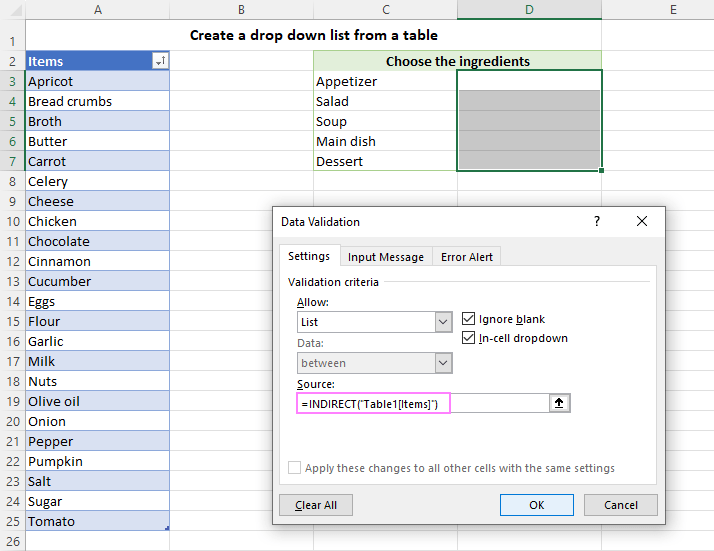
For this example, we are going to use the table with the plain name Table1, which resides in A2:A25 in the screenshot below. To make a picklist from this table, the steps are:
- Select one or more cells for your dropdown (D3:D7 in our case).
- On the Data tab, in the Data Tools group, click Data Validation.
- In the Allow drop-down box, select List.
- In the Source box, enter the formula that indirectly refers to Table1’s column named Items. =INDIRECT("Table1[Items]")
- When done, click OK.
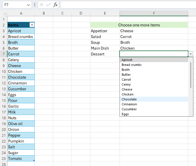
The result will be an expandable and automatically updatable drop-down list that only allows selecting one item.
Tip. If the method described above is not suitable for you for some reason, you can create a dropdown from a regular range or named range.
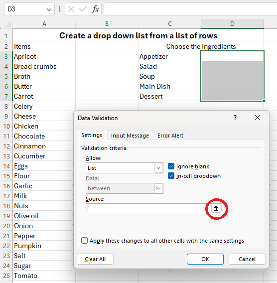
Creating a drop down list without using a table
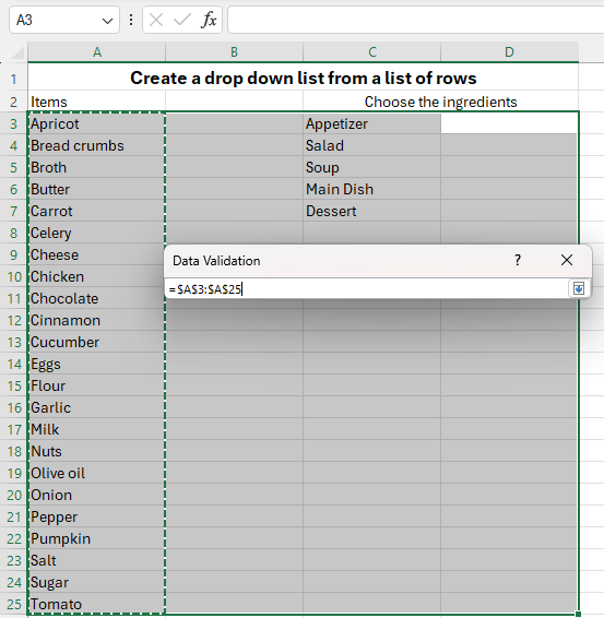
Similar to the process above, you don’t have to put the data in a table. You can just create a list in rows and then use the Data Validation and instead of using a formula for the Source, you can select the up arrow on Source and select the range.
Tables are better because they are dynamic. As you add more data, the ranges increase automatically. However, you can get away without making it a table.
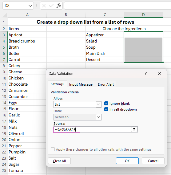
Tip: If you want the drop down list to have a title, make certain to include the name of your list i.e. Items. The cell will show blank until you use the drop down. It would be recommended to put borders around your cells to identify the drop down list as the arrows do not show until you click the cell.
If you want Blank to be an option, include an extra row in the list and uncheck Ignore blank.
Disappearing List
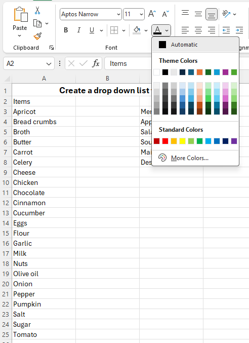
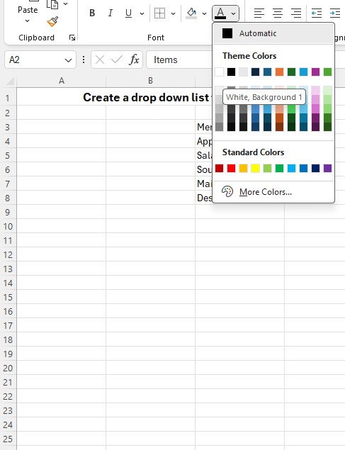
If you want just the drop down list but not the list it is referencing, you can hide the list in a different location on the sheet or the workbook. Just make sure that the Source is pointing to the range. Then you can change the color of the font of the list to White so it doesn’t appear against a White background.
Related Articles
Microsoft Excel: How to make pivot charts
Microsoft Excel: How to make pivot charts The tutorial shows how to quickly create, filter and customize pivot charts in Excel, so you can make the most of your data. If you’ve ever felt overwhelmed by a large and cluttered spreadsheet, you’re not ...Microsoft Excel: How to select rows and columns
Microsoft Excel: How to select rows and columns In this article, we will guide you through various methods to select rows and columns in Excel, including some helpful shortcuts. Efficiency is the name of the game when it comes to Excel. Selecting ...Microsoft Excel: Add a combo box to a worksheet
Microsoft Excel: Add a combo box to a worksheet When you want to display a list of values that users can choose from, you can add a combo box to your worksheet. Note: If your Excel Ribbon does not have the Developer tab do the following; Click File > ...Microsoft Excel: Header and Footer – Insert, Edit and Remove
Microsoft Excel: Header and Footer – Insert, Edit and Remove To make your printed Excel documents look more stylish and professional, you can include a header or footer on each page of your worksheet. Generally, headers and footers contain basic ...Microsoft Excel: Text to Columns
Microsoft Excel: Text to Columns Data imported from other spreadsheets or databases is already separated into fields, using something called a field delimiter: a comma, tab, space, or custom character – to separate one field from another. These ...