Microsoft Excel: How to select alternate columns
Microsoft Excel: How to select alternate columns
This article will guide you step-by-step through the process of selecting specific columns in Excel, such as every other or every nth column.
Microsoft Excel, the go-to spreadsheet software for data enthusiasts and professionals, offers several methods to select columns based on specific criteria.
Select alternate columns in Excel
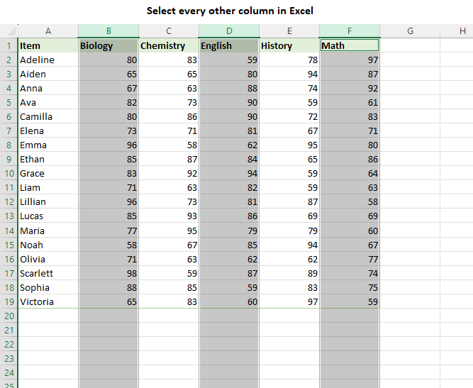
The simplest way to select alternate columns in Excel is by utilizing the Ctrl key in combination with the mouse. Here’s how you can do it:
- Press and hold the Ctrl key on your keyboard.
- While holding the Ctrl key, click on the header of every other column.
- Repeat steps 2 and 3 until you have selected all the desired columns.
- Release the Ctrl key.
As a result, you have the alternate columns selected:
By using the Ctrl key, you can handpick every 3rd, every 4th or every nth column, so you can apply formatting or perform calculations on specific sections of your data.
This method of selecting every other or every nth column is a straightforward and effective approach, particularly for small datasets. However, it may become cumbersome and time-consuming when dealing with large sets of data. Manually clicking on each column header can be prone to errors and can become tiresome. In such cases, alternative methods come in handy to streamline the process and save valuable time.
Selecting every other or nth column with a formula
If you prefer a more precise method to select every other or nth column in Excel, you can achieve this by using the CHOOSECOLS function. Here’s how you can use it:
- In an empty cell, enter the CHOOSECOLS formula. The first argument should be the source range that contains the columns you want to select.
- In the subsequent arguments, provide the column numbers you want to return.
- Press Enter to apply the formula.
- For example, to select every even column in the range A2:F20, the formula takes this form:
=CHOOSECOLS(A2:F20, 2, 4, 6)
This formula specifies that you want to return columns 2, 4, and 6 from the range A2:F20.
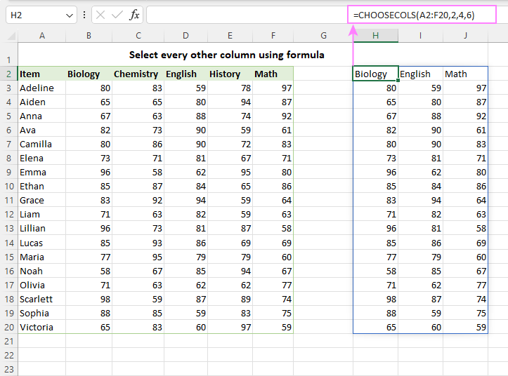
The CHOOSECOLS formula returns the specified columns as a dynamic array, which you can easily select and copy to another part of your worksheet.
Related Articles
Microsoft Excel: Text to Columns
Microsoft Excel: Text to Columns Data imported from other spreadsheets or databases is already separated into fields, using something called a field delimiter: a comma, tab, space, or custom character – to separate one field from another. These ...Microsoft Excel: How to select rows and columns
Microsoft Excel: How to select rows and columns In this article, we will guide you through various methods to select rows and columns in Excel, including some helpful shortcuts. Efficiency is the name of the game when it comes to Excel. Selecting ...Microsoft Excel: How to freeze Rows & Columns
Microsoft Excel: How to freeze Rows & Columns Freeze the Top Row or First Column Click on the View tab on the Excel Ribbon. Click the drop-down for Freeze Panes. Click Freeze Top Row – allows scrolling down many rows and still shows the top row. OR ...Microsoft Excel: How to print row and column headers on every page
Microsoft Excel: How to print row and column headers on every page In printing spreadsheets; the top row is printed only on the first page. Here is how to repeat the header row on your print jobs. Repeat Excel header rows on every page Your Excel ...Microsoft Excel: Concatenation (Concat)
Microsoft Excel: Concatenation (Concat) Concatenation – What is it? The CONCAT function is one of Excel’s text functions. It is used to join two or more columns of text from multiple ranges and/or strings, but it doesn’t provide delimiter or ...